Neuron network is about mimicking the brain. Our brain can learn anything with one algorithm (“one learning algorithm” hypothesis, re-wiring test).

How our brain works

A neuron takes inputs from other neurons or sensors, process and provide outputs to other neurons. The way we learn is to change the weight of each input for output.

Neuron Model: Logistic Unit

For each neuron, with input of , output would be . Here, is the activation function(whether this neuron output a big value).

Artificial Neural Network

Activation Function (Hypothesis Function)

To justify, activation function is not hypothesis function since there should be only one hypothesis function. Activation function of the output layer is the hypothesis function.

Vectorized:

Remember to add biased unit

Cost Function

Cost function of neural network is just summing up cost function of logistic regression for each output unit.
For the regularization part, just sum up all the parameters except for the bias units.

Optimization

Forward-propagation

Execute activation function (and adding bias unit) for each layer.

Back-propagation

Back-propagation is to calculate how much to
For output layer units:

For hidden layer units:

where

Multiclass classification

• One-vs-all: Output layer has n units each represent a class

Random Initialization

To make each neuron unit get different features, we should initialize the randomly (in ).
A good choice of is

Notations

• : “activation”(output) of unit in layer
• : matrix storing all parameters (weights) that the neurons in layer uses to get output.
• : No. of layers
• : No. of units(not include bias unit) in layer
• : No. of units in output layer

How Normal Equation Works?

Solve for analytically.

Pros

• No need to choose
• No need feature scaling
• Don’t need to iterate

Cons

• Slow when having a lot of features (not using when )

Algorithm

• : Design matrix, takes all input data (including )

Algorithm:
set to 0

Result:

Non-invertible

In matlab/octave, pinv() will handle the case.

Causes of non-invertible:

• Redundant features (linearly dependent)
  • Delete one of the dependent feature
• Too many features (e.g. )
  • Delete some features
  • Regularization

How Gradient Descent Works?

Start with a initial parameter set:
Keep changing the parameter set to reduce
Until we hopefully end up at a minimum.
Declare convergence if decreases by less than in one iteration.

Pros

• Works well even when a lot of features.
• Simple

Cons

• Needs many iterations.
• Slow

Algorithm

• : learning rate

repeat until convergence {

}

Note: should update all parameters simultaneously.

Normalization

See regularization

Gradient Checking (numerical gradient)

To identify/debug error(usually back-propagation in neural network), we need to check whether the gradient is calculated correctly. (Should not be on when learning)

$
\frac{d}{d\Theta_i}J(\Theta)\approx \frac{J(\Theta_i+\epsilon, \Theta_{rest})-J(\Theta_i-\epsilon, \Theta_{rest})}{2\epsilon}

$

usually with

Different Types of Gradient Descent

“Batch” Gradient Descent

Each step of gradient descent uses all the training samples.
It could be computational expensive to sum all errors.

Stochastic Gradient Descent

1. Randomly shuffle dataset
2. Update for each sample
   It goes randomly, ends up wondering around local optimum.

Mini-Batch Gradient Descent

1. Randomly shuffle dataset
2. Update for each samples
   Somewhere in between batch gradient descent and stochastic gradient descent.

*Advantage than stochastic gradient descent: by using vectorization, calculation could be done faster

Preprocessing

Feature Scaling

Make sure features are on a similar scale, so that we can choose a more proper learning rate.

Usually, get every feature into approximately a

Mean Normalization

Replace with to make features have approximately zero mean (do not apply to )

If is increasing or waving

should decrease after every iteration.
Use smaller

Combine Features

Just combine features into new features directly.

Polynomial Regression

Just create new features like and to achieve polynomial regression.

Online Courses for machine learning

The machine learning course from Stanford in coursera is a great and famous resource to learn machine learning. If you want to start learning machine learning, even if you got no foundation, you should take a look at it.

What is Machine learning?

Machine learning is about using data to get a model that can describe and predict data.
Machine learning includes supervised learning and unsupervised learning.

• Supervised learning is a machine learning which training data are labeled.
• unsupervised learning is a machine learning which training data are not labeled.

Regression, Supervised

Outputs are real numbers.

Minimization Algorithms:

• Gradient Descent
• Conjugate Gradient
• BFGS
• L-BFGS

Linear Regression

Check out Linear Regression

Classification, Supervised

Outputs are discrete(0, 1, 2 ……).

• Two-class classification
• Multi-class classification
  • One-vs-all(one-vs-rest): make a classifier for each class

Clustering, Unsupervised

Output cluster centroids, giving clusters by distance to the centroids

• K-means

Logistic Regression

Check out Logistic Regression

Clustering, Unsupervised

Over-fitting

Model perform accurate on training model, but do not generalize

Solutions:

1. Reduce number of features
   • Manually select which features to keep
   • Model selection algorithm
2. Regularization
   • Penalize by adding to cost function, where is regularization parameter. (Do not penalize )

Notations

• : Number of training samples
• : “input” variables
• : “output” variables
• : i-th sample
• : j-th column of i-th sample
• : parameters of the model
• : hypothesis function that takes input to estimate output.
• : cost function that takes parameters to calculate the accuracy of prediction from hypothesis function.

Introduction

ERD was first proposed by Peter Chen in 1976

Components

Entities

Entity Type is represented capitalised using a rectangular box.

Attributes

Attributes is represented using ellipse.

Primary Key

Represented by underlining the name of the attribute.

Multi-valued Attribute

Represented using concentric ellipses

Derived Attribute

Represented using a dashed ellipse

Relationships

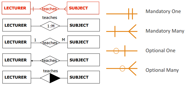
Relationship is represented using a diamond

Cardinality

Cardinality describes how many entities are related in each side.

Can be:

• One-to-One
• One-to-Many
• Many-to-Many

Participation

Participation Constraint is presented by min:max indicating number of times an entity can participate in a relationship.

• Total
  All entities should participate in at lease one relationship.
• Partial

Other Entities

Associative Entity

Entity used to associate many to many relationship wile storing other attributes.

Represented as both entity and relationship - diamond in a rectangle.

Weak Entity

Weak entity is an entity depend on another entity.

Represented using double rectangle.

Syntax

PHP Code

1
2
3

<?php
    ...
?>

Note All statements end with a semicolon ;
Note Everything except variable names are NOT case sensitive.

Comments

// and # are used for single-line comment
/* ... */ can be used for multi-line comment

Variables

Usage

$variable_name = "anything"

Note: PHP is a loosely typed language

Scope

• local
• global
• static

Global

global keyword can be used to make variable global.
$GLOBALs['index'] can be used to access global variables.

Static

Static variable is local. It won’t be deleted when function completed.
static keyword can be used to make variable static.

Constant

1
2

define("SHI", "Hello world!"[, case_insensitive = false]);
echo SHI;

Data Type

var_dump($x); can be used to show the type of a variable.

String

Variables can be integrated directly into strings:

1

echo "<h1>$txt</h1>";

Note: echo and print can be used with or without parentheses

. can be used to concatenate strings.
.= to append.

Array

1
2
3
4
5
6
7
8

$a = array(1, 2, 3);
$a[0];

$b = array("a"=>1, "b"=>2, "c"=>3);
$b['a'];
foreach($b as $bi => $bi_value) {
    echo "Key=" . $bi . ", Value=" . $bi_value;
}

Function

1
2
3
4

function fu($a, $b=0) {
    ...
    return 0
}

Object

1
2
3
4
5
6
7
8
9
10

class Bi {
    function Bi(){
        $this->shi = "shi";
    }
}

// Create an object
$b = new Bi();

echo $b->shi;

Condition Statement

If

1
2
3
4
5
6
7

if() {
    ...
} elseif() {
    ...
} else{
    ...
}

Switch

1
2
3
4
5
6
7
8

switch (n) {
    case label1:
        ...
        break;
    ...
    default:
        ...
}

Loops

While

1
2
3
4
5
6
7

while() {
    ...
}

do {
    ...
} while();

For

1
2
3
4
5
6
7

for(...;...;...) {
    ...
}

for ($i as $arr) {
    ...
}

Skills

Redirection

1
2

header("Location: ".$url, true, $permanent ? 301 : 302);
die();

First order

Separable

Separate and integrate both sides

Linear

Standard form:

Second order

Linear Homogeneous

Standard form:

Assume: ( may be real or complex)

Since , and

So the solution:

• Two real
• Two complex
• One real

Two complex

As is complex numbers, they can be rewritten as

Using Euler’s theorem,

One real

Coupled DE

Coupled Linear DE with constant coefficients

Differentiate (1) wrt (make it second order derivative of wrt )

Substitute for and (getting rid of )

Solve DE wrt

Get Form Data

1
2

$_GET["field"]
$_POST["field"]

Validation

Not empty

1
2
3

if (empty($_POST["field"])) {
  $err = "Field is required";
}

Letters and white space only

1
2
3

if (!preg_match("/^[a-zA-Z ]*$/",$field)) {
  $err = "Only letters and white space allowed"; 
}

E-mail address

1
2
3

if (!filter_var($email, FILTER_VALIDATE_EMAIL)) {
  $err = "Invalid email format"; 
}

Url

1
2
3

if (!preg_match("/\b(?:(?:https?|ftp):\/\/|www\.)[-a-z0-9+&@#\/%?=~_|!:,.;]*[-a-z0-9+&@#\/%=~_|]/i",$url)) {
  $err = "Invalid URL"; 
}